A Taste of dplyr 1.0.0

A quick summary of some exciting features coming in dplyr 1.0, e.g. across(), row-wise operations and context-dependent expressions

6/2/2020

15 min read

49 views

Last modified: 11/9/2024

Note This article has been updated to keep up with dplyr 1.1.

This post uses the penguins dataset modified by Allison Horst in all the code examples (as an alternative to iris).

library(dplyr)
#> Attaching package: 'dplyr'
#> The following objects are masked from 'package:stats':
#> 
#>     filter, lag
#> The following objects are masked from 'package:base':
#> 
#>     intersect, setdiff, setequal, union
library(ggplot2)

packageVersion("dplyr")
#> [1] '1.1.2'

penguins <- palmerpenguins::penguins
penguins

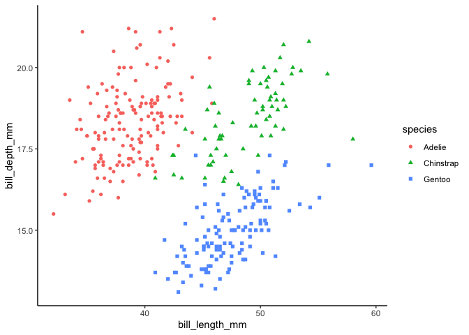
penguins %>%
  ggplot(aes(bill_length_mm, bill_depth_mm, color = species, shape = species)) +
  geom_point()
#> Warning: Removed 2 rows containing missing values or values outside the scale range
#> (`geom_point()`).
#> Warning in vp$just: partial match of 'just' to 'justification'

Column-wise Workflows

The new across() function supersedes functionalities of _at, _if, _all variants. The first argument, .cols, selects the columns you want to operate on. It uses tidy selection (like select()) so you can pick variables by position, name, and type. The second argument, .fns, is a function or list of functions to apply to each column. This can also be a purrr style formula

penguins_grouped <- penguins %>% group_by(species)

penguins_grouped %>%
  summarize(across(starts_with("bill"), ~ mean(.x, na.rm = TRUE)),
    n = n()
  )
#>   species   bill_length_mm bill_depth_mm     n
#>   <fct>              <dbl>         <dbl> <int>
#> 1 Adelie              38.8          18.3   152
#> 2 Chinstrap           48.8          18.4    68
#> 3 Gentoo              47.5          15.0   124

For conditional selection (previous _if variants), predicate function should be wrapped in where.

# double all numeric columns
penguins %>%
  mutate(across(where(is.numeric), ~ .x * 2))
# count unique values of all character columns
penguins %>%
  summarize(across(where(is.character), ~ length(unique(.x))))
#> # A tibble: 1 × 0

Apply multiple functions using list and use the .names argument to control column names.

penguins_grouped %>%
  summarize(across(matches("mm"),
    list(
      min = ~ min(.x, na.rm = TRUE),
      max = ~ max(.x, na.rm = TRUE)
    ),
    .names = "{fn}_{col}"
  ))
#>   species   min_bill_length_mm max_bill_length_mm min_bill_depth_mm
#>   <fct>                  <dbl>              <dbl>             <dbl>
#> 1 Adelie                  32.1               46                15.5
#> 2 Chinstrap               40.9               58                16.4
#> 3 Gentoo                  40.9               59.6              13.1
#> # ℹ 3 more variables: max_bill_depth_mm <dbl>, min_flipper_length_mm <int>,
#> #   max_flipper_length_mm <int>

Row-wise Workflows

Row-wise operations require a special type of grouping where each group consists of a single row. You create this with rowwise().

df <- tibble(
  student_id = 1:4,
  test1 = 10:13,
  test2 = 20:23,
  test3 = 30:33,
  test4 = 40:43
)
df %>% rowwise()
#> # Rowwise: 
#>   student_id test1 test2 test3 test4
#>        <int> <int> <int> <int> <int>
#> 1          1    10    20    30    40
#> 2          2    11    21    31    41
#> 3          3    12    22    32    42
#> 4          4    13    23    33    43

rowwise doesn’t need any additional arguments unless you have variables that identify the rows, like student_id here. This can be helpful when you want to keep a row identifier.

Like group_by, rowwise doesn’t really do anything itself; it just changes how the other verbs work.

df %>% mutate(avg = mean(c(test1, test2, test3, test4)))
#>   student_id test1 test2 test3 test4   avg
#>        <int> <int> <int> <int> <int> <dbl>
#> 1          1    10    20    30    40  26.5
#> 2          2    11    21    31    41  26.5
#> 3          3    12    22    32    42  26.5
#> 4          4    13    23    33    43  26.5

df %>%
  rowwise() %>%
  mutate(avg = mean(c(test1, test2, test3, test4)))
#> # Rowwise: 
#>   student_id test1 test2 test3 test4   avg
#>        <int> <int> <int> <int> <int> <dbl>
#> 1          1    10    20    30    40    25
#> 2          2    11    21    31    41    26
#> 3          3    12    22    32    42    27
#> 4          4    13    23    33    43    28

rowwise takes each row, feeds it into a function, and return a tibble with the same number of rows. This essentially parallelize a function over the rows in the dataframe. In this case, the mean() function is vectorized. But, if a function is already vectorized, then rowwise is not needed.

df %>% mutate(s = test1 + test2 + test3)
#>   student_id test1 test2 test3 test4     s
#>        <int> <int> <int> <int> <int> <int>
#> 1          1    10    20    30    40    60
#> 2          2    11    21    31    41    63
#> 3          3    12    22    32    42    66
#> 4          4    13    23    33    43    69

df %>%
  rowwise() %>%
  mutate(s = test1 + test2 + test3)
#> # Rowwise: 
#>   student_id test1 test2 test3 test4     s
#>        <int> <int> <int> <int> <int> <int>
#> 1          1    10    20    30    40    60
#> 2          2    11    21    31    41    63
#> 3          3    12    22    32    42    66
#> 4          4    13    23    33    43    69

Another family of summary functions have “parallel” extensions where you can provide multiple variables in the arguments:

df %>%
  mutate(
    min = pmin(test1, test2, test3, test4),
    max = pmax(test1, test2, test3, test4),
    string = paste(test1, test2, test3, test4, sep = "-")
  )
#>   student_id test1 test2 test3 test4   min   max string     
#>        <int> <int> <int> <int> <int> <int> <int> <chr>      
#> 1          1    10    20    30    40    10    40 10-20-30-40
#> 2          2    11    21    31    41    11    41 11-21-31-41
#> 3          3    12    22    32    42    12    42 12-22-32-42
#> 4          4    13    23    33    43    13    43 13-23-33-43

Where these functions exist, they’ll usually be faster than rowwise. The advantage of rowwise is that it works with any function, not just those that are already vectorized.

However, an advantage of rowwise even there is other ways is that it’s paired with c_across(), which works like c() but uses the same tidyselect syntax as across(). That makes it easy to operate on multiple variables:

df %>%
  rowwise() %>%
  mutate(
    min = min(c_across(starts_with("test"))),
    max = max(c_across(starts_with("test")))
  )
#> # Rowwise: 
#>   student_id test1 test2 test3 test4   min   max
#>        <int> <int> <int> <int> <int> <int> <int>
#> 1          1    10    20    30    40    10    40
#> 2          2    11    21    31    41    11    41
#> 3          3    12    22    32    42    12    42
#> 4          4    13    23    33    43    13    43

Plus, a rowwise df will naturally contain exactly the same rows after summarize(), the same as mutate

df %>%
  rowwise() %>%
  summarize(across(starts_with("test"), ~ .x, .names = "{col}_same"))
#>   test1_same test2_same test3_same test4_same
#>        <int>      <int>      <int>      <int>
#> 1         10         20         30         40
#> 2         11         21         31         41
#> 3         12         22         32         42
#> 4         13         23         33         43

List Columns

Because lists can contain anything, you can use list-columns to keep related objects together, regardless of what type of thing they are. List-columns give you a convenient storage mechanism and rowwise gives you a convenient computation mechanism.

df <- tibble(
  x = list(1, 2:3, 4:6),
  y = list(TRUE, 1, "a"),
  z = list(sum, mean, sd)
)
df
#>   x         y         z     
#>   <list>    <list>    <list>
#> 1 <dbl [1]> <lgl [1]> <fn>  
#> 2 <int [2]> <dbl [1]> <fn>  
#> 3 <int [3]> <chr [1]> <fn>

df %>%
  rowwise() %>%
  summarize(
    x_length = length(x),
    y_type = typeof(y),
    z_call = z(1:5)
  )
#>   x_length y_type    z_call
#>      <int> <chr>      <dbl>
#> 1        1 logical    15   
#> 2        2 double      3   
#> 3        3 character   1.58

Simulation

The basic idea of using rowwise to perform simulation is to store all your simulation parameters in a data frame, similar to purrr::pmap.

df <- tribble(
  ~id, ~n, ~min, ~max,
  1, 3, 0, 1,
  2, 2, 10, 100,
  3, 2, 100, 1000,
)

Then you can either generate a list-column containing the simulated values with mutate:

df %>%
  rowwise() %>%
  mutate(sim = list(runif(n, min, max)))
#> # Rowwise: 
#>      id     n   min   max sim      
#>   <dbl> <dbl> <dbl> <dbl> <list>   
#> 1     1     3     0     1 <dbl [3]>
#> 2     2     2    10   100 <dbl [2]>
#> 3     3     2   100  1000 <dbl [2]>

Or taking advantage of summarize’s new features to return multiple rows per group

df %>%
  rowwise(everything()) %>%
  summarize(sim = runif(n, min, max))

Note

In dplyr 1.1, you should use reframe() instead of summarize() to return multiple rows.

df |>
  rowwise(everything()) |>
  reframe(sim = runif(n, min, max))

Without rowwise, you would need to use purrr::pmap to perform the simulation.

df %>%
  mutate(sim = purrr::pmap(., ~ runif(..2, ..3, ..4)))
#>      id     n   min   max sim      
#>   <dbl> <dbl> <dbl> <dbl> <list>   
#> 1     1     3     0     1 <dbl [3]>
#> 2     2     2    10   100 <dbl [2]>
#> 3     3     2   100  1000 <dbl [2]>

Group-wise Models

The new nest_by() function works similarly to group_nest()

by_species <- penguins %>% nest_by(species)
by_species
#> # Rowwise:  species
#>   species                 data
#>   <fct>     <list<tibble[,7]>>
#> 1 Adelie             [152 × 7]
#> 2 Chinstrap           [68 × 7]
#> 3 Gentoo             [124 × 7]

Now we can use mutate to fit a model to each data frame:

by_species <- by_species %>%
  rowwise(species) %>%
  mutate(model = list(lm(bill_length_mm ~ bill_depth_mm, data = data)))

by_species
#> # Rowwise:  species
#>   species                 data model 
#>   <fct>     <list<tibble[,7]>> <list>
#> 1 Adelie             [152 × 7] <lm>  
#> 2 Chinstrap           [68 × 7] <lm>  
#> 3 Gentoo             [124 × 7] <lm>

And then extract model summaries or coefficients with summarize() and broom functions (note that by_species is still a rowwise data frame):

by_species %>%
  summarize(broom::glance(model))
by_species %>%
  summarize(broom::tidy(model))

An alternative approach

penguins %>%
  group_by(species) %>%
  group_modify(~ broom::tidy(lm(bill_length_mm ~ bill_depth_mm, data = .x)))
#> # Groups:   species [3]
#>   species   term          estimate std.error statistic  p.value
#>   <fct>     <chr>            <dbl>     <dbl>     <dbl>    <dbl>
#> 1 Adelie    (Intercept)     23.1       3.03       7.60 3.01e-12
#> 2 Adelie    bill_depth_mm    0.857     0.165      5.19 6.67e- 7
#> 3 Chinstrap (Intercept)     13.4       5.06       2.66 9.92e- 3
#> 4 Chinstrap bill_depth_mm    1.92      0.274      7.01 1.53e- 9
#> 5 Gentoo    (Intercept)     17.2       3.28       5.25 6.60e- 7
#> 6 Gentoo    bill_depth_mm    2.02      0.219      9.24 1.02e-15

New `summarize` Features

Note

Use reframe() instead of summarize() to return multiple rows starting from dplyr 1.1.

Multiple Rows and Columns

Two big changes make summarize() much more flexible. A single summary expression can now return:

A vector of any length, creating multiple rows. (so we can use summary that returns multiple values without list)
A data frame, creating multiple columns.

penguins_grouped %>%
  summarize(
    bill_length_dist = quantile(bill_length_mm,
      c(0.25, 0.5, 0.75),
      na.rm = TRUE
    ),
    q = c(0.25, 0.5, 0.75)
  )

Or return multiple columns from a single summary expression:

penguins_grouped %>%
  summarize(tibble(
    min = min(bill_depth_mm, na.rm = TRUE),
    max = max(bill_depth_mm, na.rm = TRUE)
  ))
#>   species     min   max
#>   <fct>     <dbl> <dbl>
#> 1 Adelie     15.5  21.5
#> 2 Chinstrap  16.4  20.8
#> 3 Gentoo     13.1  17.3

At the first glance this may seem not so different with supplying multiple name-value pairs. But this can be useful inside functions. For example, in the previous quantile code it would be nice to be able to reduce the duplication so that we don’t have to type the quantile values twice. We can now write a simple function because summary expressions can now be data frames or tibbles:

quibble <- function(x, q = c(0.25, 0.5, 0.75), na.rm = TRUE) {
  tibble(x = quantile(x, q, na.rm = na.rm), q = q)
}

penguins_grouped %>%
  summarize(quibble(bill_depth_mm))

When combining glue syntax and tidy evaluation, it is easy to dynamically name the column names.

quibble <- function(x, q = c(0.25, 0.5, 0.75), na.rm = TRUE) {
  tibble(
    "{{ x }}_quantile" := quantile(x, q, na.rm = na.rm),
    "{{ x }}_q" := q
  )
}

penguins_grouped %>%
  summarize(quibble(flipper_length_mm))

As an aside, if we name the tibble expression in summarize() that part will be packed in the result, which can be solved by tidyr::unpack. That’s because when we leave the name off, the data frame result is automatically unpacked.

penguins_grouped %>%
  summarize(df = quibble(flipper_length_mm))

Non-summary Context

In combination with rowwise operations, summarize() is now sufficiently powerful to replace many workflows that previously required a map() function.

For example, to read all the all the .csv files in the current directory, you could write:

tibble(path = dir(pattern = "\\.csv$")) %>%
  rowwise(path) %>%
  summarize(read_csv(path))

Move Columns

New verb relocate is provided to change column positions with the same syntax as select. The default behavior is to move selected columns to the left-hand side

penguins %>% relocate(island)
penguins %>% relocate(starts_with("bill"))
penguins %>% relocate(sex, body_mass_g, .after = species)

Similarly, mutate gains new arguments .after and .before to control where new columns should appear.

penguins %>%
  mutate(mass_double = body_mass_g * 2, .before = 1)

Row Mutations

dplyr has a new experimental family of row mutation functions inspired by SQL’s UPDATE, INSERT, UPSERT, and DELETE. Like the join functions, they all work with a pair of data frames:

rows_update(x, y) updates existing rows in x with values in y.
rows_patch(x, y) works like rows_update() but only changes NA values.
rows_insert(x, y) adds new rows to x from y.
rows_upsert(x, y) updates existing rows in x and adds new rows from y.
rows_delete(x, y) deletes rows in x that match rows in y.

The rows_ functions match x and y using keys. All of them check that the keys of x and y are valid (i.e. unique) before doing anything.

df <- tibble(a = 1:3, b = letters[c(1:2, NA)], c = 0.5 + 0:2)
df
#>       a b         c
#>   <int> <chr> <dbl>
#> 1     1 a       0.5
#> 2     2 b       1.5
#> 3     3 <NA>    2.5

We can use rows_insert() to add new rows:

new <- tibble(a = c(4, 5), b = c("d", "e"), c = c(3.5, 4.5))

rows_insert(df, new)
#> # A tibble: 5 × 3
#>       a b         c
#>   <int> <chr> <dbl>
#> 1     1 a       0.5
#> 2     2 b       1.5
#> 3     3 <NA>    2.5
#> 4     4 d       3.5
#> 5     5 e       4.5

Note that rows_insert() will fail if we attempt to insert a row that already exists:

df %>% rows_insert(tibble(a = 3, b = "c"))
#> Matching, by = "a"
#> Error in `rows_insert()`:
#> ! `y` can't contain keys that already exist in `x`.
#> ℹ The following rows in `y` have keys that already exist in `x`: `c(1)`.
#> ℹ Use `conflict = "ignore"` if you want to ignore these `y` rows.

df %>% rows_insert(tibble(a = 3, b = "c"), by = c("a", "b"))
#>       a b         c
#>   <int> <chr> <dbl>
#> 1     1 a       0.5
#> 2     2 b       1.5
#> 3     3 <NA>    2.5
#> 4     3 c      NA

If you want to update existing values, use rows_update(). It will throw an error if one of the rows to update does not exist:

df %>% rows_update(tibble(a = 3, b = "c"))
#> # A tibble: 3 × 3
#>       a b         c
#>   <int> <chr> <dbl>
#> 1     1 a       0.5
#> 2     2 b       1.5
#> 3     3 c       2.5

df %>% rows_update(tibble(a = 4, b = "d"))
#> Matching, by = "a"
#> Error in `rows_update()`:
#> ! `y` must contain keys that already exist in `x`.
#> ℹ The following rows in `y` have keys that don't exist in `x`: `c(1)`.
#> ℹ Use `unmatched = "ignore"` if you want to ignore these `y` rows.

rows_patch() is a variant of rows_update() that will only update values in x that are NA.

df %>% rows_patch(tibble(a = 1:3, b = "patch"))
#> # A tibble: 3 × 3
#>       a b         c
#>   <int> <chr> <dbl>
#> 1     1 a       0.5
#> 2     2 b       1.5
#> 3     3 patch   2.5

row_upsert update a df or insert new rows.

df %>%
  rows_upsert(tibble(a = 3, b = "c")) %>% # update
  rows_upsert(tibble(a = 4, b = "d")) # insert
#> Matching, by = "a"
#> # A tibble: 4 × 3
#>       a b         c
#>   <int> <chr> <dbl>
#> 1     1 a       0.5
#> 2     2 b       1.5
#> 3     3 c       2.5
#> 4     4 d      NA

Context Dependent Expressions

n() is a special function in dplyr which return the number of observations in the current group. Now the new version comes with more such special functions, aka context dependent expressions. These functions return information about the “current” group or “current” variable, so only work inside specific contexts like summarize() and mutate(). Specifically, a family of cur_ functions are added:

cur_data() gives the current data for the current group (excluding grouping variables, cur_data_all in developmental version returns grouping variables as well)
cur_group() gives the group keys, a tibble with one row and one column for each grouping variable.
cur_group_id() gives a unique numeric identifier for the current group
cur_column() gives the name of the current column (in across() only).

Note

cur_data() is deprecated in favor of pick(col1, col2, ...) in dplyr 1.1.

df <- tibble(
  g = sample(rep(letters[1:3], 1:3)),
  x = runif(6),
  y = runif(6)
)
gf <- df %>% group_by(g)

gf %>% reframe(row = cur_group_rows())
#>   g       row
#>   <chr> <int>
#> 1 a         4
#> 2 b         5
#> 3 b         6
#> 4 c         1
#> 5 c         2
#> 6 c         3
gf %>% reframe(data = list(cur_group()))
#> # A tibble: 3 × 2
#>   g     data            
#>   <chr> <list>          
#> 1 a     <tibble [1 × 1]>
#> 2 b     <tibble [1 × 1]>
#> 3 c     <tibble [1 × 1]>
gf %>% reframe(data = list(pick(everything())))
#>   g     data            
#>   <chr> <list>          
#> 1 a     <tibble [1 × 2]>
#> 2 b     <tibble [2 × 2]>
#> 3 c     <tibble [3 × 2]>

# cur_column() is not related to groups
gf %>% mutate(across(everything(), ~ paste(cur_column(), round(.x, 2))))
#> # Groups:   g [3]
#>   g     x      y     
#>   <chr> <chr>  <chr> 
#> 1 c     x 0.84 y 0.59
#> 2 c     x 0.56 y 0.52
#> 3 c     x 0.08 y 0.16
#> 4 a     x 0.96 y 0.28
#> 5 b     x 0.02 y 0.6 
#> 6 b     x 0.32 y 0.1

Superseded Functions

top_n(), sample_n(), and sample_frac() have been superseded in favor of a new family of slice helpers: slice_min(), slice_max(), slice_head(), slice_tail(), slice_random().

# select penguins per group on body mass
penguins_grouped %>%
  slice_max(body_mass_g, n = 1)
#> # Groups:   species [3]
#>   species   island bill_length_mm bill_depth_mm flipper_length_mm body_mass_g
#>   <fct>     <fct>           <dbl>         <dbl>             <int>       <int>
#> 1 Adelie    Biscoe           43.2          19                 197        4775
#> 2 Chinstrap Dream            52            20.7               210        4800
#> 3 Gentoo    Biscoe           49.2          15.2               221        6300
#> # ℹ 2 more variables: sex <fct>, year <int>

penguins_grouped %>%
  slice_min(body_mass_g, n = 1)
#> # Groups:   species [3]
#>   species   island bill_length_mm bill_depth_mm flipper_length_mm body_mass_g
#>   <fct>     <fct>           <dbl>         <dbl>             <int>       <int>
#> 1 Adelie    Biscoe           36.5          16.6               181        2850
#> 2 Adelie    Biscoe           36.4          17.1               184        2850
#> 3 Chinstrap Dream            46.9          16.6               192        2700
#> 4 Gentoo    Biscoe           42.7          13.7               208        3950
#> # ℹ 2 more variables: sex <fct>, year <int>

# random sampling
penguins %>%
  slice_sample(n = 10)
penguins %>%
  slice_sample(prop = 0.1)

summarize() gains new argument .groups to control grouping structure of theh result.

.groups = "drop_last" drops the last grouping level (i.e. the default behaviour).
.groups = "drop" drops all grouping levels and returns a tibble.
.groups = "keep" preserves the grouping of the input.
.groups = "rowwise" turns each row into its own group.

Other Changes

The new rename_with() makes it easier to rename variables programmatically:

penguins %>%
  rename_with(stringr::str_to_upper)

You can optionally choose which columns to apply the transformation to with the second argument:

penguins %>%
  rename_with(stringr::str_to_upper, starts_with("bill"))

mutate() gains argument .keep that allows you to control which columns are retained in the output:

penguins %>% mutate(
  double_mass = body_mass_g * 2,
  island_lower = stringr::str_to_lower(island),
  .keep = "used"
)
penguins %>% mutate(double_mass = body_mass_g * 2, .keep = "none")

Recipes

This in-progress section documents tasks that would otherwise been impossible or laborious with previous version of dplyr.

Replace Missing Values in Multiple Columnes

Since tidyr::replace_na does not support tidy select syntax, replacing NA values in multiple columns could be a drudgery. Now this is made easy with coalesce and across

penguins %>% summarize(across(starts_with("bill"), ~ sum(is.na(.x))))
#> # A tibble: 1 × 2
#>   bill_length_mm bill_depth_mm
#>            <int>         <int>
#> 1              2             2

penguins %>%
  mutate(across(starts_with("bill"), ~ coalesce(.x, 0))) %>%
  summarize(across(starts_with("bill"), ~ sum(is.na(.x))))
#> # A tibble: 1 × 2
#>   bill_length_mm bill_depth_mm
#>            <int>         <int>
#> 1              0             0

Rolling Regression

We can easily perform rolling computation with the slider package and pick().

library(slider)
library(lubridate)
#> 
#> Attaching package: 'lubridate'
#> The following objects are masked from 'package:base':
#> 
#>     date, intersect, setdiff, union
# historical stock prices from 2014-2018 for Google, Amazon, Facebook and Apple
stock <- tsibbledata::gafa_stock %>% select(Symbol, Date, Close, Volume)
stock

# Arrange and group by `Symbol` (i.e. Google)
stock <- stock %>%
  arrange(Symbol, Date) %>%
  group_by(Symbol)

linear_model <- function(df) {
  lm(Close ~ Volume, data = df)
}

# 10 day rolling regression per group
stock %>%
  mutate(model = slide_index(
    pick(Close, Volume),
    Date,
    linear_model,
    .before = days(9),
    .complete = TRUE
  ))

Column-wise Workflows

Row-wise Workflows

List Columns

Simulation

Group-wise Models

New summarize Features

Multiple Rows and Columns

Non-summary Context

Move Columns

Row Mutations

Context Dependent Expressions

Superseded Functions

Other Changes

Recipes

Replace Missing Values in Multiple Columnes

Rolling Regression

New `summarize` Features